Creating your first ggrank plot • ggrank

ggrank shows how categories move through an ordered ranking while retaining their underlying values. Start with one row per category and period and map the three required columns.

Teaching-data notice: All datasets bundled with ggrank are synthetic. They do not contain Global Burden of Disease estimates. ggrank is an independent project and is not affiliated with or endorsed by the Institute for Health Metrics and Evaluation (IHME).

library(ggrank)

ggrank(
  ggrank_products,
  category = product,
  period = year,
  value = sales,
  periods = c(2022, 2024),
  top_n = 5,
  value_header = "Sales"
)

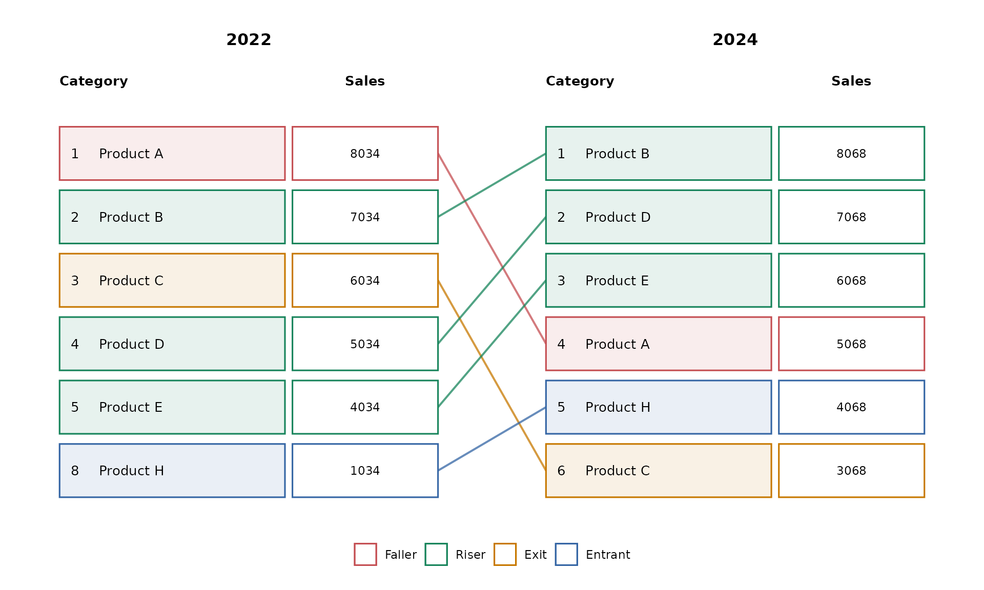
The boundary view is the default: a category outside the top five remains in the figure when it enters or exits the top five in another displayed period.

Let ggrank calculate the ranks

Users normally supply values rather than ranks. Inspect the calculation with ggrank_data():

tied_rates <- data.frame(
  year = rep(c(2020, 2025), each = 5),
  organism = rep(c("A", "B", "C", "D", "E"), 2),
  rate = c(5, 4, 3, 3, 2, 6, 4, 4, 2, 1)
)

ggrank_data(
  tied_rates,
  category = organism,
  period = year,
  value = rate
)
#>    category period value rank display_position label group
#> 1         A   2020     5    1                1     5  <NA>
#> 2         B   2020     4    2                2     4  <NA>
#> 3         C   2020     3    3                3     3  <NA>
#> 4         D   2020     3    3                4     3  <NA>
#> 5         E   2020     2    5                5     2  <NA>
#> 6         A   2025     6    1                1     6  <NA>
#> 7         B   2025     4    2                2     4  <NA>
#> 8         C   2025     4    2                3     4  <NA>
#> 9         D   2025     2    4                4     2  <NA>
#> 10        E   2025     1    5                5     1  <NA>

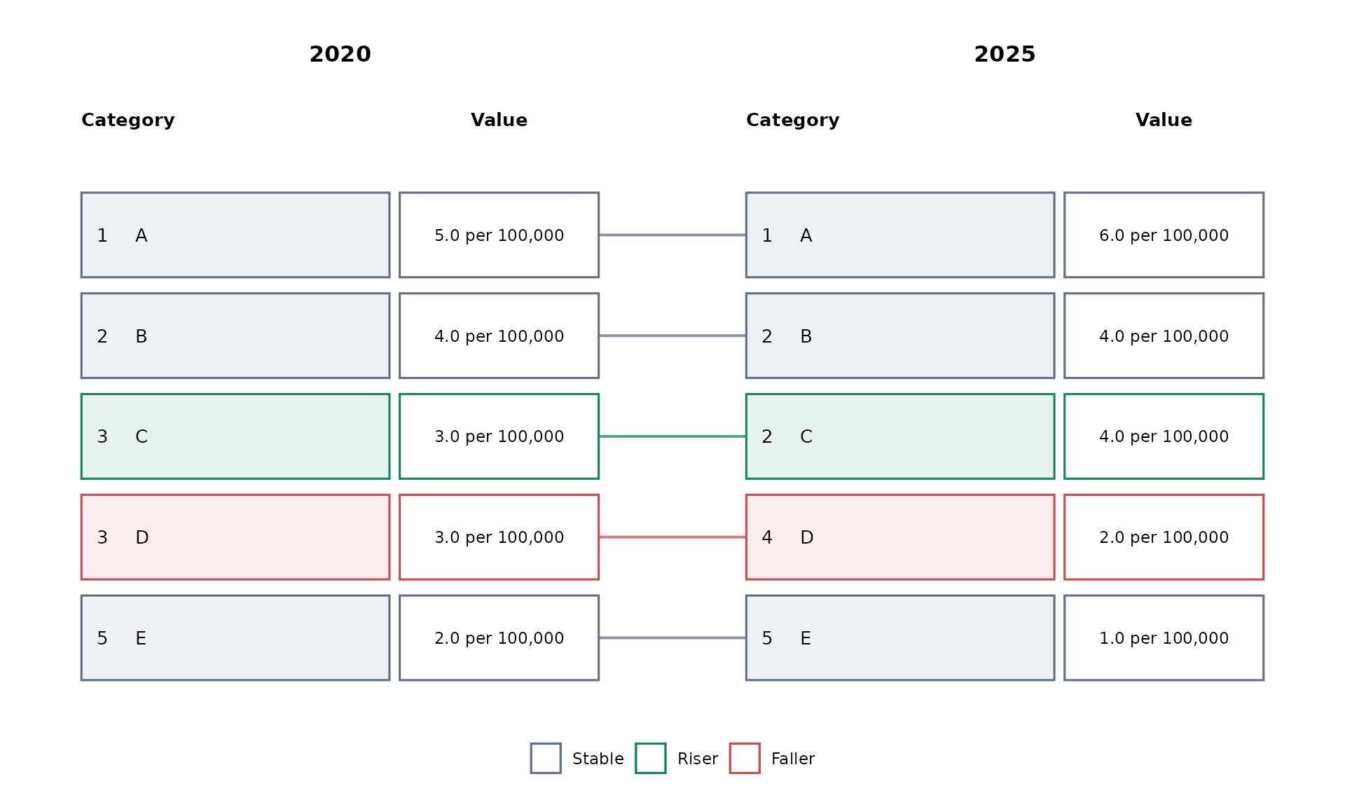
Ranking uses exact numeric values. Equal values share a competition rank by default (1, 2, 3, 3, 5) but receive separate alphabetical display positions. All categories tied at the top_n boundary are included, so a top-ten figure can contain more than ten boxes. Do not filter to the top N before calling the package, because doing so prevents entrant and exit detection.

Display formatting is independent of ranking. For example, rank an unrounded rate while printing a prepared one-decimal label:

formatted_rates <- transform(
  tied_rates,
  rate_label = sprintf("%.1f per 100,000", rate)
)

ggrank(
  formatted_rates,
  category = organism,
  period = year,
  value = rate,
  label = rate_label
)

Use existing ranks without marks or values

If a school, institution, or report already supplies authoritative ranks, no mark, rate, score, or other value column is needed.

student_ranks <- data.frame(
  year = rep(c(2024, 2025), each = 4),
  student = rep(c("Asha", "Ben", "Chen", "Dina"), 2),
  institution = "North School",
  rank = c(1, 2, 3, 4, 3, 1, 2, 4)
)

ggrank(
  student_ranks,
  category = student,
  period = year,
  rank = rank,
  group = institution,
  top_n = 4
)

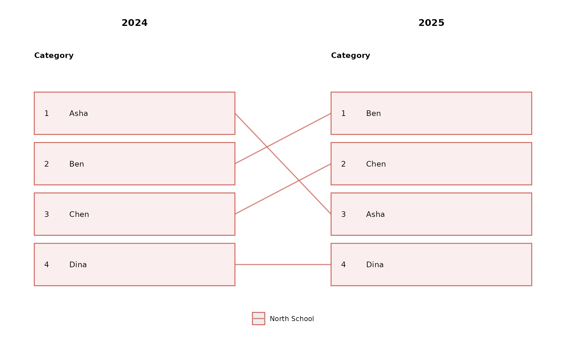
The rank-only layout omits the value boxes. The same input works with ggrank_data(), ggrank_table(), and ggrank_change(). Ranks must be finite, positive whole numbers. group changes colours; it does not calculate ranks separately for each group. Separate institutional ranking lists should be analysed separately or represented by distinct period/list identifiers.

Group colours and prepared labels

Use group for meaningful category colours and label when values require a domain-specific display format. Supplied ranks are also supported.

ggrank(
  ggrank_causes,
  category = cause,
  period = year,
  value = rate,
  rank = rank,
  label = display_value,
  group = cause_group,
  periods = c(1990, 2021),
  top_n = 10,
  value_header = "Rate (95% interval)"
)

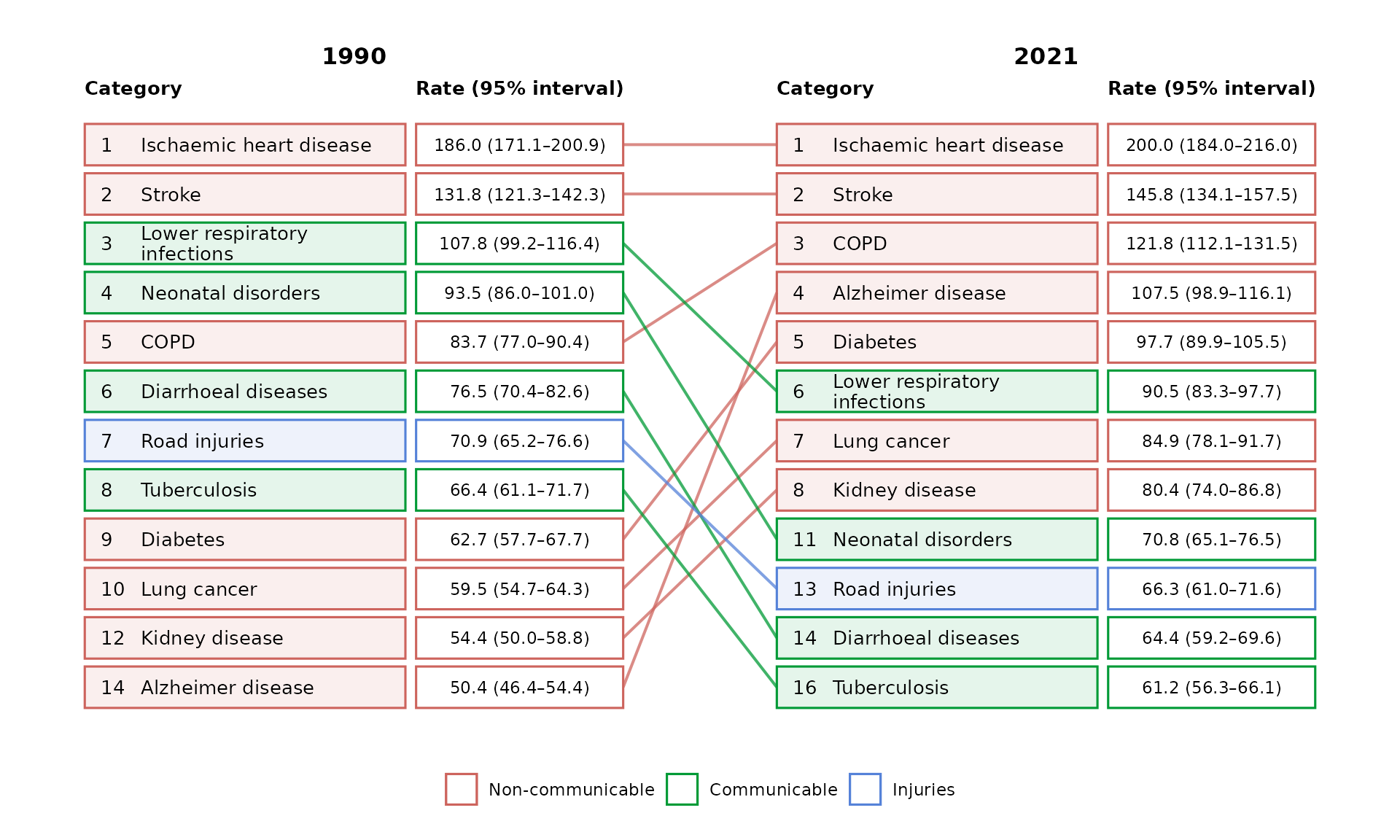
The returned value is a regular ggplot object, so titles, captions, and other ggplot2 layers can be added normally.

Inspect the underlying comparison

ggrank_table() returns a readable analytical companion with one row per category and adjacent transition.

changes <- ggrank_table(
  ggrank_products,
  category = product,
  period = year,
  value = sales,
  periods = c(2022, 2024),
  top_n = 5
)

changes
#>    category from   to rank_from rank_to rank_change value_from value_to
#> 1 Product B 2022 2024         2       1           1       7034     8068
#> 2 Product D 2022 2024         4       2           2       5034     7068
#> 3 Product E 2022 2024         5       3           2       4034     6068
#> 4 Product A 2022 2024         1       4          -3       8034     5068
#> 5 Product H 2022 2024         8       5           3       1034     4068
#> 6 Product C 2022 2024         3       6          -3       6034     3068
#>   value_change label_from label_to group missing_from missing_to  status
#> 1         1034       7034     8068  <NA>        FALSE      FALSE   riser
#> 2         2034       5034     7068  <NA>        FALSE      FALSE   riser
#> 3         2034       4034     6068  <NA>        FALSE      FALSE   riser
#> 4        -2966       8034     5068  <NA>        FALSE      FALSE  faller
#> 5         3034       1034     4068  <NA>        FALSE      FALSE entrant
#> 6        -2966       6034     3068  <NA>        FALSE      FALSE    exit

Visualise the largest rises and falls directly from that table. Positive values moved towards rank one; negative values moved away from rank one.

ggrank_change(changes, top = 5)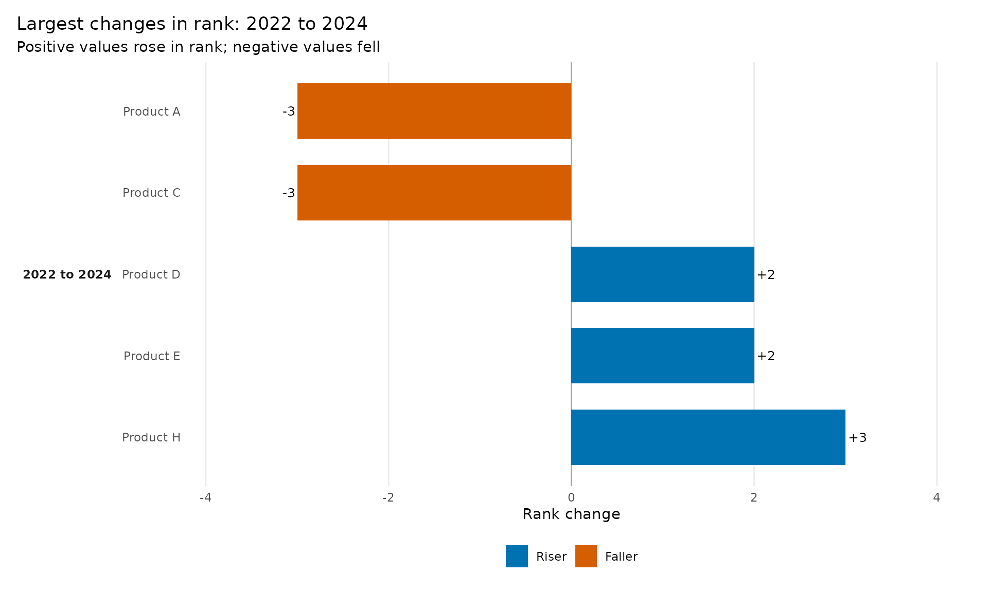

Use the graphical interface

Launch the optional local Shiny interface when you prefer to choose columns and settings interactively:

ggrank_app()

Start with either synthetic teaching dataset or upload a CSV. The GUI presents the rank chart, change chart, analytical table, and calculated rank data in separate tabs. Close the Shiny window or stop the R process to return to the console.